

The load simulator is not a simple “send N orders” tool. It models the shape of real traffic — orders are spaced out to match the historical hourly distribution, so the pressure on FIRE mirrors what happens during an actual lunch rush or evening peak.
Purpose
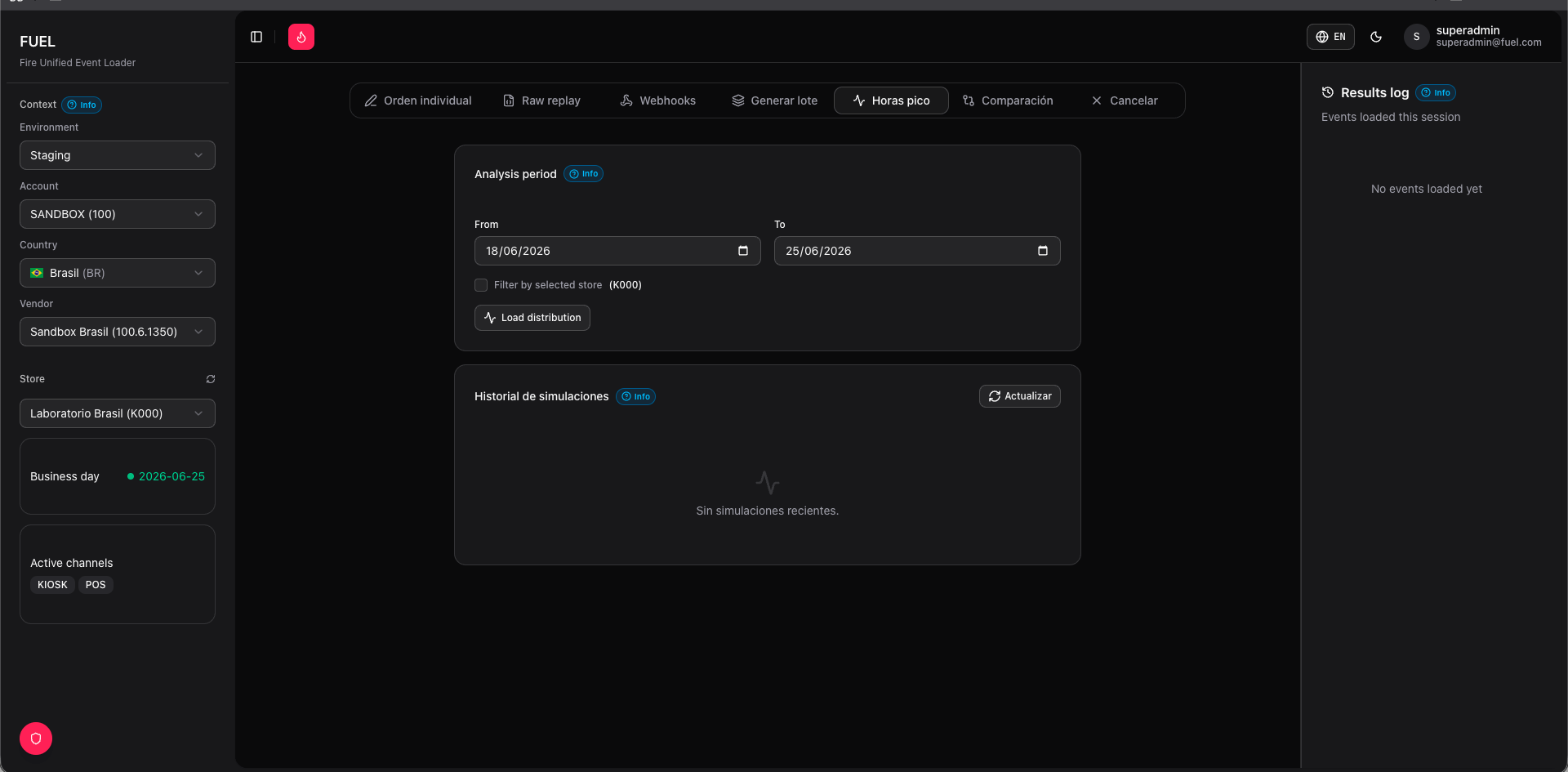
Use the Load Sim tab to stress-test FIRE under realistic conditions. Rather than flooding the system with all orders at once, the simulator computes when each order should fire based on a historical distribution curve, then introduces the right timing delays between requests. This makes it useful for validating queue behavior, KDS throughput, fiscal callback handling, and any system that responds to order velocity rather than just volume.Configuring the simulation
Data source
FIRE data
Pulls the historical order distribution directly from FIRE for a date range you specify. Use this when you want the simulation to reflect real traffic from a specific store or period.
Local samples
Uses order samples stored in FUEL’s own database. Useful when FIRE data is unavailable or you want a repeatable baseline dataset.
Hour filter
Restrict the distribution to a specific window of the day. For example, set From11 To 14 to isolate the lunch rush. Orders outside the selected range are excluded from the curve before the simulation is built.
Target duration
Set how long the entire simulation should take, in minutes. FUEL computes a compression factor automatically:If the source data spans a 4-hour peak and your target duration is 30 minutes, the compression factor is 8× — each real-world minute of traffic is compressed into 7.5 seconds of simulation time.A lower target duration means higher instantaneous order rate. Use this to amplify stress without needing more data.
Traffic curve chart
After selecting a source and applying the hour filter, FUEL renders a hourly bar chart showing the order distribution across the selected window. Review the curve before starting — it confirms which hours carry the most load and lets you validate that the filter captured the right period.Running the simulation
1
Configure source, hours, and duration
Select your data source, set the hour filter, and enter the target duration in minutes.
2
Review the distribution chart
Confirm the traffic curve looks correct. Adjust the hour filter if needed.
3
Click Start simulation
FUEL begins firing orders according to the compressed timeline. Orders are dispatched with the computed inter-request delays to reproduce the original shape.
4
Monitor live progress
The progress panel shows Sent, Successful, and Errors counts in real time, along with an elapsed timer and a percentage-complete indicator.
5
Stop if needed
Click Stop simulation at any point to abort. Orders already sent are not rolled back.